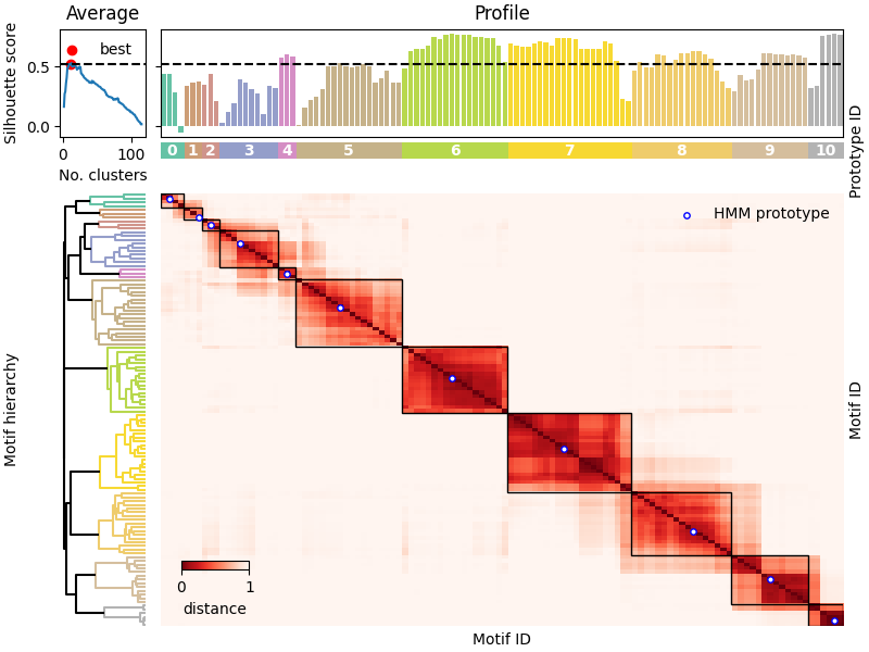
Prototype selection

Visualise the results of the prototype selection step.

We use the data from the CalMS21 Task1 dataset (Sun et al., 2021).

Import and configure modules

Import the necessary modules and configure the plotting settings.

import matplotlib.pyplot as plt
import numpy as np
from huggingface_hub import hf_hub_download
from scipy.spatial.distance import squareform

import lisbet.plotting as betp

# Configure
plt.rcParams["figure.constrained_layout.use"] = True

Fetch the sample data from HuggingFace

Fetch and load the information file containing the results of the prototype selection. This file is generated by the command betman prototype_selection.

data_path = hf_hub_download(
    repo_id="gchindemi/lisbet-examples",
    filename="prototype_selection/CalMS21_Task1/info_hmmbest_6_32.npz",
    repo_type="dataset",
)
hmm_info = np.load(data_path)

Visualise the data

Plot the silhouette profile and the prototype selection results.

fig, axs = plt.subplots(
    nrows=2,
    ncols=2,
    width_ratios=[2, 16],
    height_ratios=[4, 16],
    figsize=(8, 6),
)

# Share axes
axs[0, 0].sharey(axs[0, 1])
axs[0, 1].sharex(axs[1, 1])

# Customize layout
fig.align_ylabels(axs[:, 0])

betp.plot_slh_score(
    hmm_info["all_n_clusters"],
    hmm_info["all_score"],
    hmm_info["best_n_clusters"],
    hmm_info["best_score"],
    axs[0, 0],
)

betp.plot_slh_profile(
    distance=squareform(hmm_info["cond_dist_matrix"]),
    link_matrix=hmm_info["link_matrix"],
    cluster_labels=hmm_info["best_labels"],
    ax=axs[0, 1],
)

betp.plot_dendrogram(
    hmm_info["link_matrix"],
    cluster_labels=hmm_info["best_labels"],
    ax=axs[1, 0],
)

betp.plot_heatmap(
    squareform(hmm_info["cond_dist_matrix"]),
    hmm_info["link_matrix"],
    hmm_info["best_labels"],
    hmm_info["prototypes"],
    ax=axs[1, 1],
)

# Finalize plot
axs[0, 0].legend(frameon=False)
axs[1, 1].legend(frameon=False)

<matplotlib.legend.Legend object at 0x700dfca36e70>